Linear regression in Machine learning

With hands-on experience from my internships at Samsung R&D and Wictronix, where I worked on innovative algorithms and AI solutions, as well as my role as a Microsoft Learn Student Ambassador teaching over 250 students globally, I bring a wealth of practical knowledge to my Hashnode blog. As a three-time award-winning blogger with over 2400 unique readers, my content spans data science, machine learning, and AI, offering detailed tutorials, practical insights, and the latest research. My goal is to share valuable knowledge, drive innovation, and enhance the understanding of complex technical concepts within the data science community.
Are you seeking a resource that can teach you all there is to know about the linear regression algorithm? If so, you've come to the correct spot. You'll be equipped to work with this algorithm once you've finished reading this blog post. Let's get started without further delay.
Introduction to linear regression in machine learning
Linear regression is a machine learning algorithm that is used to solve regression problems, in which the machine learning algorithm predicts a continuous numerical value for a single input or set of inputs. There are three forms of linear regression: simple linear regression, multiple linear regression, and polynomial regression.
The primary distinctions between these three types of linear regression are as follows:
| Simple linear regression | Multiple linear regression | Polynomial regression |
| It is a type of linear regression, where there is only one independent and dependent variable | It is a type of linear regression, where there are more than one independent and only one dependent variable | Polynomial Regression is a form of Linear regression known as a special case of Multiple linear regression which estimates the relationship between a dependent(y) and independent variable(x) as nth degree polynomial |
| Example: Determine whether a student will pass the exam based on the number of study hours they put in. | Example: Determine whether or not it will rain based on the temperature, humidity, and wind speed. | Example: It is widely applied to predict the spread rate of COVID-19 and other infectious diseases. |
Only linear regression will be covered in this blog post; multiple linear regression and polynomial linear regression will be covered in subsequent posts.
Simple linear regression
The primary idea behind simple linear regression is that it tries to find the best fit line, which is just a mathematical function for which the cost function value is smallest, or we may say that the difference between the actual and predicted value is minimal.
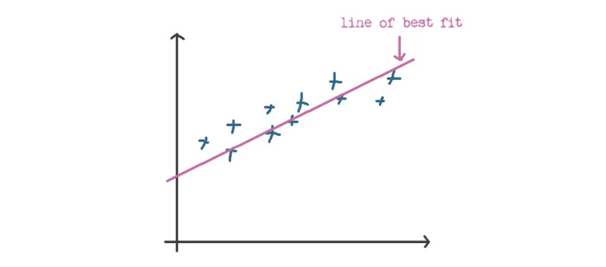
The best fit line's mathematical equation is given as y = mx + c, where y is the predicted output value, m is the slope (used to represent the rate of change of the output value with a unit change in the value of the input value), x is the input value, and c is the offset, which refers to the point where the line intersects y when x = 0.
Now, we can deduce from the mathematical formula that, to find the best fit line, the hyperparameters y and m will be crucial, because changing these two parameters will change the overall position of the best fit line.
Mathematics behind simple linear regression
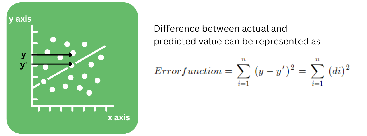
Before diving deep into the mathematics behind simple linear regression, the thing to keep in mind is that for finding the best fit line, we have to find those values of m and c for which the difference between the actual and predicted value is minimum.
Ordinary least squares (OLS) and gradient descent are two methods for determining the values of m and c for which the difference between the actual value and the anticipated value is the least.
Ordinary least squares technique for finding m and c
Now that we have carefully noticed that m and c are not present in the error function's mathematical formula, the question arises as to how we might even reduce the value of the error function. Slope (m) and offset (c) are the only two parameters that can be changed to affect the error function's value. However, since we are aware that y=mx+b represents the best fit line, employing this equation will result in the error function becoming
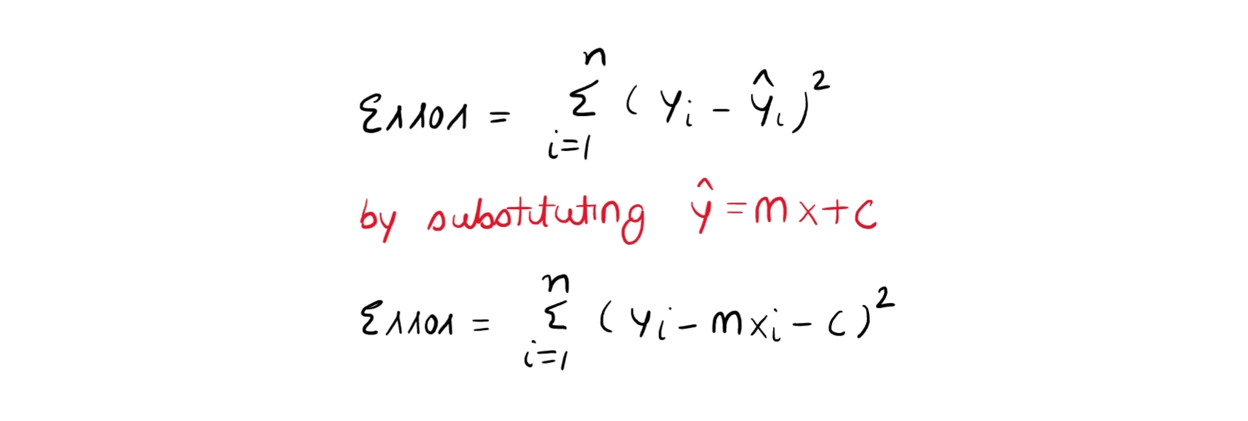
We finally have our error function after exchanging the values, so let's see how its value will change when the slope and offset variables change.

In the above visual, J(θ,θ1) represents the error function, θ represents slope, and θ represents offset.
The local maxima and minima, which are depicted by the red and blue colors in the gif above, are the places where the graph flattens out and switches from increasing to decreasing, or vice versa. A flat graph indicates that the slope is zero. Therefore, we will partially differentiate the error function about the slope and offset to get the formula for slope and offset, and we will set the result equal to 0.
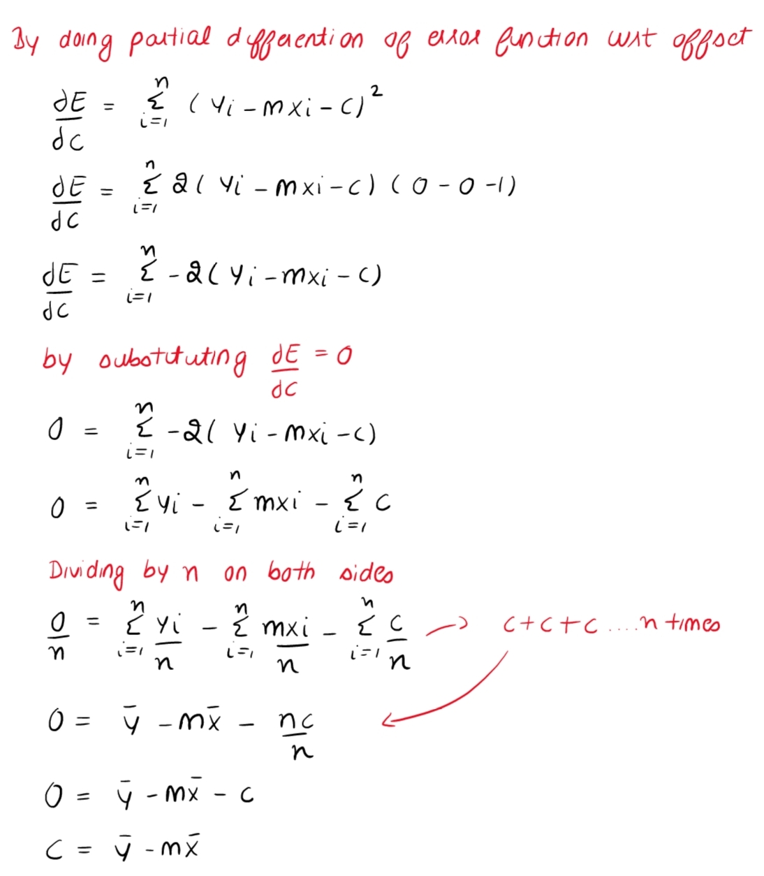
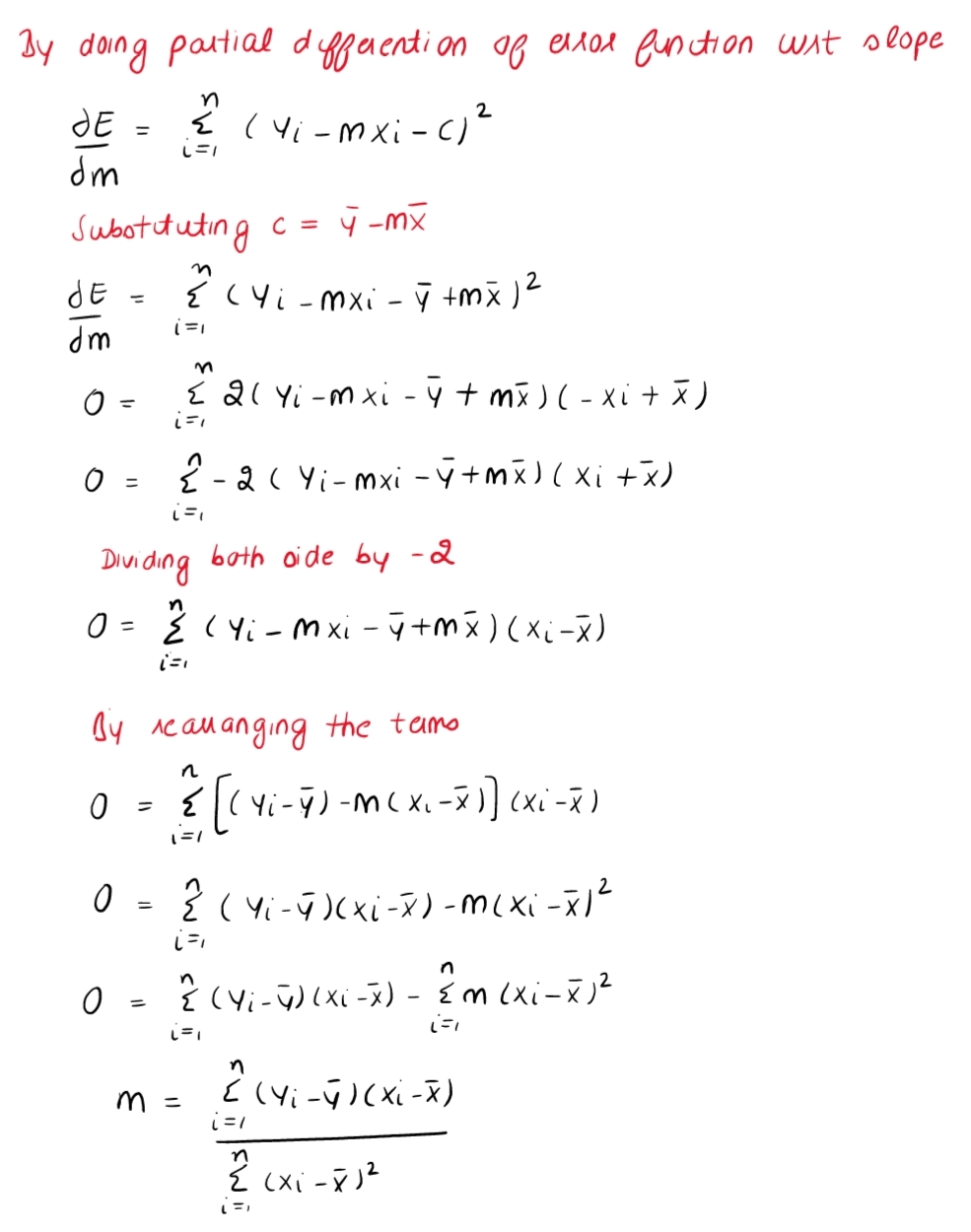
Following the partial differentiation of the error function regarding the offset, we will repeat the process, but this time about the slope.
That's all for now, and I hope this blog provided some useful information for you. Additionally, don't forget to check out my 👉 TWITTER handle if you want to receive daily content relating to data science, mathematics for machine learning, Python, and SQL.


